By Jade Philipoom
In this post, we’ll explain a new method to benchmark ML-DSA signing with relatively few test inputs. We can get a better measurement from as few as 1 or 2 specially-selected test inputs as we would get from 100 random tests. You can find the code here.
ML-DSA signing: a benchmarking challenge
ML-DSA signing time is notoriously variable and difficult to benchmark, with academic papers typically measuring 5000 or 10000 runs in order to get statistically meaningful results. To understand why, it’s important to know that the signing operation is a rejection loop: it repeatedly tries to generate a signature and then runs some checks. If a check fails, the routine rejects the candidate signature, generates a new one, and restarts from the beginning. About 75-80% of candidate signatures fail. This creates a “long tail” in the performance curve, as shown in the graph below.
The median number of loop iterations is 3 (ML-DSA-44 and ML-DSA-87) or 4 (ML-DSA-65), but a significant minority of signatures take 10 or more iterations. For benchmarks, that means the few signatures that take a very long time contribute disproportionately to the average. It’s also worth noting that due to the shape of this curve, the median will always be significantly below the mean (4.3, 5.2, or 3.9 iterations for ML-DSA-44, -65, and -87). This is why ML-DSA papers such as the Dilithium1 round 3 NIST PQC submission provide both the median and mean for signing benchmarks, not just the median as it does for other operations.
The takeaway is, if you’re measuring ML-DSA performance from just a few tests, then your average cycle count will depend heavily on how many long-running inputs you happened to sample, rather than the actual performance characteristics of your code.
For us at ZeroRISC, this posed a challenge: to get cycle-accurate measurements, we need to run on slow hardware-simulation platforms like Verilator or block-specific simulators, where a single ML-DSA signature generation can take a minute or more. We also want to run these measurements relatively often to avoid accidental performance regressions and to give others an accurate sense of the expected performance. But at one minute per test and with 3 parameter sets to check, running even 100 tests on each parameter set would take five hours, and running 10000 would take 500 hours! (In fact, researchers we collaborate with recently had to do this monster run of 10K tests for their publication; it took days to complete on a heavily parallelized university computing cluster.) We needed a way to characterize the performance of the signing routine without burning so much compute time.
Cleverly selecting inputs
Facing this problem, I remembered a blog post from Filippo Valsorda that I’d read some time ago. In that post, he addresses a similar challenge in benchmarking RSA key generation, which also has a long rejection loop construction to find random primes. I encourage you to read his post for the full details, but the basic idea is to look at the different points in the code where a particular implementation might reject values (typically trial divisions or Miller-Rabin), mathematically calculate the percentage of values that should be rejected at each point, and then come up with a list of numbers that gets rejected from each point at rates that are close to average.
This idea extends, with a little bit of modification, to ML-DSA. (After drafting this post, I spoke to Filippo about it at RWC 2026 and it turns out that he had independently implemented and applied a very similar approach for the Go crypto library!) The Dilithium specification has mathematical formulas for how many candidate signatures should get rejected from each condition. But unlike RSA key generation where rejections are determined by divisibility by certain numbers, there aren’t really elegant mathematical formulas to tell us exactly which candidate signatures will fail a “znorm” check. We have to actually run the code. For this purpose, I somewhat hackily modified the ML-DSA reference code’s test-vector generation code to also print out a byte string with each test vector that traces iterations of the sign loop and where they stopped. Using this new feature, I collected a sample of 100,000 pseudorandom test inputs. Speed isn’t a huge issue here, thankfully, since the code runs in C instead of using slow hardware simulations; generating the 100,000 signatures with rejection traces on my laptop took only a few minutes.
Equipped with my large augmented dataset, I now needed to find a way to pick specific sets of n test inputs, for any given value of n, such that the profile of sign loop iterations was as close as possible to average. I ended up choosing a simple greedy algorithm here:
- Start with an empty list of test inputs as the benchmarking set.
- Split the preprocessing dataset into n chunks.
- For each chunk, try adding each test input in turn to the benchmarking set, and measure the absolute distance of the observed pass rates of all rejection points to their known average pass rates. Add the test input that minimizes that distance to the benchmarking set.
The tests that get picked depend on the order of the preprocessed test inputs. Therefore, to pseudorandomly generate different sets of tests, you can shuffle the preprocessed dataset at the start, which is handy.
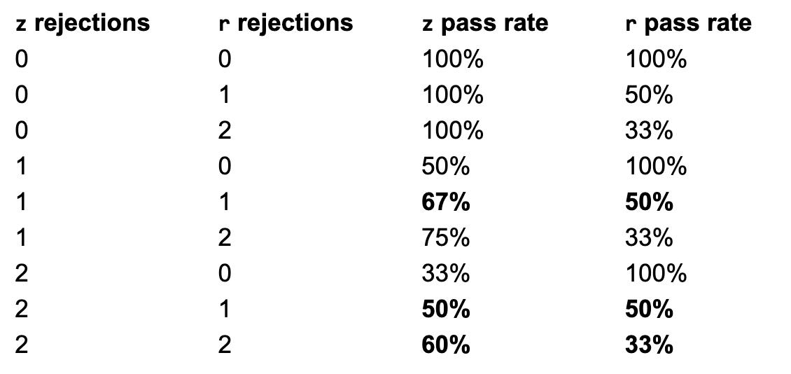
One other bit of trivia: the profile of the different algorithms, as well as the sample size, influences how close it’s possible to sample to the average performance profile. The following table summarizes the pass rates of each rejection condition for possible execution traces, with the ones that are “close to average” in bold. We only consider the z and r rejection conditions here because the others happen with a < 1% probability.
And here are the idealized average pass rates for each parameter set, and their best match among those options:
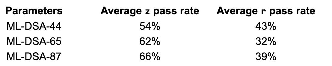
We can see from these two tables that ML-DSA-65’s ideal profile is actually quite close to that of a single signing run with 2 z rejections and 2 r rejections (62%/32% vs 60%/33%). For this reason, it’s possible to get a pretty good idea of ML-DSA-65 mean signing performance from a single well-chosen test.
ML-DSA-44 is not so lucky, with its closest match being 2 z rejections and 1 r rejection (50%/50% vs an ideal of 54%/43%). At first glance, ML-DSA-87 seems similarly unlucky, but it has two best matches: one rejection each (67%/50%) and two rejections each (60%/30%) that are both approximately as far off from the ideal (66%/39%) as each other and as ML-DSA-44’s best match. However, the average of these two matches is 63.5%/40%, a pretty close match. So we’d expect that, with two or more well-chosen tests, we’d see a pretty close to average profile for ML-DSA-87.
There’s some additional variation beyond what the rejection trace shows us, because the coefficient that causes the rejection can occur at any place in the polynomial (and since rejected signatures are not sensitive information, we can immediately discard and retry upon finding a bad coefficient). Therefore, having larger test sets does still somewhat increase the quality of benchmark results, particularly in memory-optimized implementations like ours where polynomials are handled one at a time and coefficient checks are interleaved with other operations.
Evaluation
To determine how well my sampling method worked, I repeatedly ran benchmarking runs of different sizes with either randomly-selected inputs or inputs specially chosen as described above. Then, I plotted the mean cycle counts from each benchmarking run – in other words, the value you’d think represented your ML-DSA signing performance if that was the only benchmarking run you did. Ideally, you’d want those mean numbers to be pretty close together. As expected, however, running 10 random tests produces wildly varying results (the tall columns in the graph below).
Depending on your luck with test selection on a 10-test dataset, you might think your ML-DSA-87 implementation signs in 800 kilocycles or 1600 – a factor of two difference. The standard deviation of these 10 averages of 10 random tests each is about 20% of their mean (a relative standard deviation of 20%). Even ML-DSA-44, which has the narrowest range in this sample of 10 sets of 10 random tests, has a relative standard deviation of about 17%2. Running 100 tests narrows things down, but the range of mean values is still pretty wide; in my sample of 10 sets of 100 random tests each, the relative standard deviation ranged from 5% for ML-DSA-87 to 9% for ML-DSA-65.
Selecting tests cleverly, however, gives us a much narrower range of expected results. We can also see that the selected tests look accurate, as well as precise; they tend to cluster near the mean of the 10 means from 100 random tests, meaning that the results of the selected tests are at least close to the mean of 1000 random tests. Even with only 10 runs per benchmarking set, the averages of each set are close to each other, with relative standard deviations of 2-4% for all parameter sets. In other words, 10 selected tests are giving us significantly better precision than 100 random tests!
We can also zoom in on each parameter set to see how the results converge, this time including some datasets with 1 sample per benchmarking run (so each datapoint represents a single test) or 2 samples:
The single-test runs show reasonably good precision (although they are slightly affected by things like the placement of the rejected coefficient that the test set doesn’t control for). However, they have lower accuracy than runs with 10 tests, with the level of offset depending on the parameter set. You can see that lower accuracy reflected as the “1 selected” bar being positioned significantly off-center compared to benchmarking runs with more tests. This is because with only 1 test, the test selection always picks the single rejection profile that is closest to its ideal, but this single profile is often off the mark. With more tests, it’s possible to average them into something that is more accurate.
Going back to our discussion of rejection probabilities earlier in this post, you can see clearly that ML-DSA-65 has higher accuracy because the 2 z rejection and 2 r rejection profile is very close to its ideal, while ML-DSA-44 and ML-DSA-87 lose accuracy with only 1 test because the single-test profiles available are less close. With even 2 tests, the accuracy improves significantly, because the test selection can pick two inputs that average close to the ideal profile.
We can also see reflected in these single-parameter graphs the same general pattern as in the first large graph: selected tests are more precise than random tests, with good accuracy and drastically reduced standard deviations.
Extension to percentiles
The results above are all about getting accurate measurements of the mean, but what if you want to measure the median? Or the 95th percentile performance? These large-percentile measurements are important for ML-DSA because of the long tail on signing time. For example, if you’re trying to calculate what the timeout for ML-DSA signatures should be in your system, or you’re running an ML-DSA signature as part of your boot flow, you will need to know what kind of timings are within “normal range” despite being much longer than average.
I extended the scripts experimentally to cover this case, relying on the same basic infrastructure as the mean measurements. Calculating the target pass rates for each check is a bit trickier than with the mean, because we can’t just use the average pass rate of each check. Instead, we need pass rates that represent a specific slice of the distribution of execution times.
Let’s step into an idealized algorithmic world for a moment. We can imagine a long list of all the possible distinct paths that a signature could take through the checks, a path being for example “rejected at r0, rejected at z, then passed on the third iteration”. If we could order these paths by their execution time, we could step through the list and, for each path, calculate its probability and add to an accumulator. At each step, the accumulator then represents the total chance that a randomly chosen signature would have followed one of the processed paths so far. Eventually, adding to the accumulator would exceed the target percentile – at that point, we can stop and use the path we stopped on as the target profile for rejection traces.
There are two issues with the idealized method described above. First, how do we get the paths in order by execution time? Which takes longer, a trace that is rejected at the first check twice before passing or a trace that is rejected at the last check once before passing? The answer is that it depends on the implementation! For example, some implementations need to do a bunch of computation before the first check due to memory optimizations, and the relative time between checks is going to look very different than implementations that don’t do this. Whether an implementation uses hardware or software SHAKE computations will also dramatically affect the proportion of time spent between the checks.
Fortunately, just one measurement of a passing sign loop iteration is enough to measure the relative execution time between checks for a specific implementation. We can solve the problem by incorporating a “cost model” that gives these ratios, and use that model for our ordering. For example, if the cost model says that the time between the start of the loop and the first check is five times as long as the time between the first check and the second check, then a path that is rejected at the first check twice before passing will be ordered after a path that that is rejected at the second check once before passing. However, if the time between the first check and the second check is five times as long as the time between the start of the loop and the first check, the ordering would be the other way around. These values can be approximate; they’re just a heuristic. Unfortunately, it means that implementations may need to update the cost model occasionally as they change, and the same cost model might not translate well across implementations, which is important to keep in mind.
The second problem is that the trace-simulation algorithm described above is very slow. There are a lot of possible paths, especially for high percentiles. The key observation that saves us here is that we don’t actually care about the order of rejections that happen before signature acceptance; z, z, r is equivalent to z, r, z. For the probability and pass rate calculations, all we need is the count of how many rejections happened at each check.
By iterating through possible counts, not possible full traces, we can speed up the algorithm significantly. However, we then have to do a little bit of extra math when we calculate the probability. All individual paths that share rejection counts have the same total probability, since loop iterations are independent. However, different combinations of rejection counts have different numbers of individual paths that share that ordering; there is only one possible order of z, z, z, but there are 3 possible orderings of z, z, r and 6 possible orderings of z, r, h. So, we need to somehow get the number of possible orderings and then multiply it with the path probability to get the total probability of paths with a certain rejection count profile. Luckily, the number of possible orderings of a list with repetitions turns out to be a well-studied math problem with a convenient formula. With that tweak, we have performant generation of test sets that target a given percentile!
If you want to experiment with these scripts yourself, all the code is here. There are also pre-generated test sets for mean, median, 5th and 95th percentiles, although for the reasons outlined above your cost model may vary from ours for the non-mean measurements. We hope you find these useful for benchmarking your favorite ML-DSA implementation, or perhaps that you simply understand the performance profile and considerations a bit better.
Interested in learning more? Sign up for our early-access program or contact us at info@zerorisc.com.
1Dilithium was the name for ML-DSA before it was selected and standardized by NIST.
2 Part of the reason the standard deviation range for ML-DSA-44 looks smaller than the others on the graph is simply that the numbers involved are all smaller.